Image Smoothing Algorithms
During my eternal quest to knowledge, I went accross this article: http://blog.geveo.com/Image-Smoothing-Algorithms
I have a lot of personal projects (I mean, quiiiiiite a lot). So I may experiment a few things and read a lot of technical contents.
Lastly, I wanted to know how image smoothing algorithms work in spite of my poor math knowledge. One (programmer) does not simply speak maths on a daily basis. I’ve even heard that some so-called software developers do hate maths (especially the one who graduaded on Udemy after three months).
Well it’s time to make our hands dirty here, because we are going to explore maths and, above all, code.
As I was not satisfied with the work of the person who wrote the article I mentioned above, I will explore on my own what the image smoothing algorithms are all about.
Bear with me and le’t get started.
A little bit of litterature
In math, there is the notion of “kernel” which can be mistaken with the known kernel mathematical object. In image processing, it’s basically a matrix; but as programmers let’s say two dimensional array. As an example :
\[\begin{equation*} \begin{bmatrix} 1 & 2 & 3 \\ 2 & 1 & 2 \\ 3 & 2 & 1 \end{bmatrix} \end{equation*}\]The matrix above is a 3x3 matrix. It’s as if we had a list of lists in Python:
matrix = [[1, 2, 3], [2, 1, 2], [3, 2, 1]]
But why are we talking matrixes here? Because pictures are a matrix of pixels.
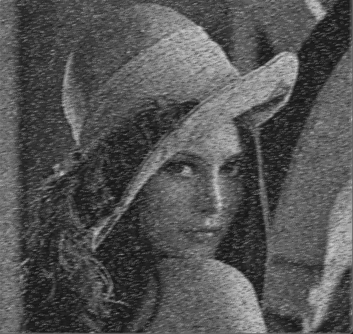
Let’s take the picture our article took in example:
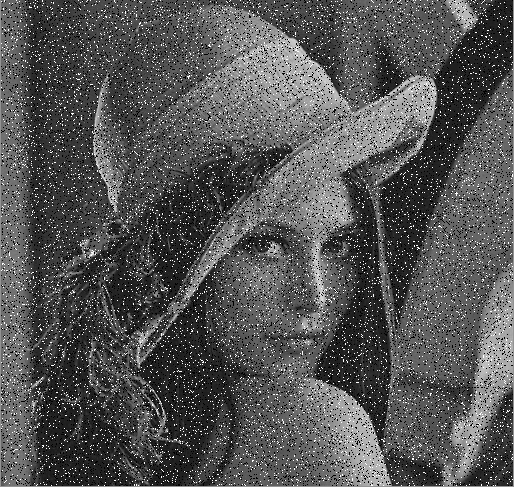
You can observe on this picture that there are a lot of black and white pixels we would like to get rid of. These unwanted pixels are called “noise”, and the image smoothing algorithms we are going to study aims at mitigating (deleting indeed) this noise.
Anyway. Let’s dig into the different algorithms.
Mode Filter Algorithm
The Mode Filter Algorithm consists in getting the “mode” of the close pixels, then pick this pixel to smooth the image.
And there you go: “what the heck is a mode?”.
In maths (again!), the mode [of a matrix] is the term which appears the most in this matrix. That’s as simple as that (and I spent way, way too much time grasping this concept).
See our matrix above? Let me paste it right here:
\[\begin{equation*} \begin{bmatrix} 1 & 2 & 3 \\ 2 & 1 & 2 \\ 3 & 2 & 1 \end{bmatrix} \end{equation*}\]Here, you can see that the term “2” appears four times, whereas the term “1” appears three times and the term “3” appears twice. So the mode of the matrix above is “2”.
And that’s how the mode filter algorithm work!
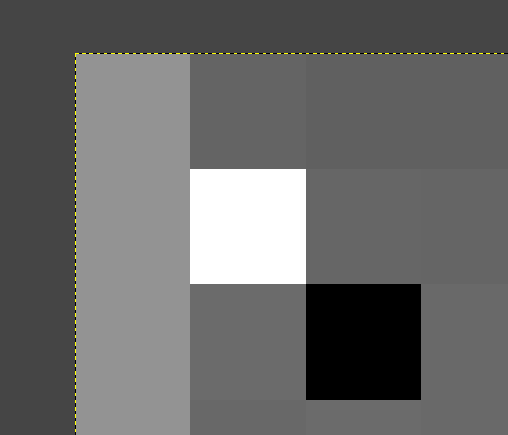
Now let’s practice a little bit, shall we? Download the picture above (it should be called “filter-me.png”) and get the first three pixels of the very first three rows, at the very top left of the picture. You may use GIMP for that.
What is helpful is that the image is at grayscale, so every level of red, green and blue in a single pixel are indentical.
Here is a screenshot of the pixels I am talking about, while I am extracting them on GIMP:
We have:
\[\begin{equation*} \begin{bmatrix} 147 & 100 & 96 \\ 147 & 255 & 102 \\ 147 & 107 & 0 \end{bmatrix} \end{equation*}\]So what’s our mode going to be here? Well, as you can see, the term “147” appears three times and is the most frequent. So the mode here is “147” and our very first pixel will have the value “147”.
I understand that this is not a relevant example, as our pixel’s grayscale is 147 already. You want a better example?
Let’s take the pixel of the second column and the second row, whose value is 255 (plain white!).
Now, let’s take the pixels around, going to the right and the bottom. Here is our new matrix and, as I feel cool, I even put a number of the pixels I am talking about, eh.
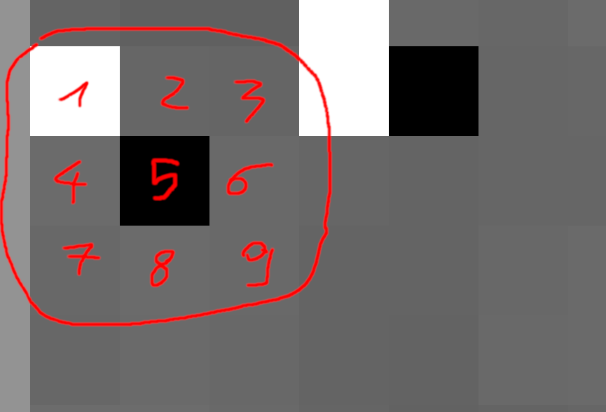
Our matrix is:
\[\begin{equation*} \begin{bmatrix} 255 & 102 & 101 \\ 107 & 0 & 105 \\ 106 & 107 & 105 \end{bmatrix} \end{equation*}\]Who’s our winner here? Well, we have an ex æequo situation, as both the terms “107” and “105” appear twice, so it’s a bimodal matrix. It has two modes. Still a bad example? Naaah… I just wanted to illustrate that not only will the value be different from 255, but also definitely far from it, regardless of whether it’s 107 or 105.
In here you can chose either modes we have come up with, so let’s stick with 105.
I hope that you have grasped the concept, so now it is time to write some python script to smooth our image using this mode algorithm thing.
Here is the content of our file called mode-filter.py.
#!/usr/bin/env python
import sys
from collections import defaultdict

from PIL import Image


def compute_mode(matrix):
    """Get the mode of the *matrix*.

    If there are more than one mode, return the first one.

    """
    occurrences = defaultdict(int)
    for element in matrix:
        occurrences[element] += 1
    return sorted(occurrences.items(), reverse=True, key=lambda a: a[1])[0][0]


def main(args):
    if len(args) < 3:
        print(f"Usage: {args[0]} IMAGE_IN IMAGE_OUT", file=sys.stderr)
        raise SystemExit(-1)

    filename_in, filename_out, *_ = args[1:]

    # Create a pillow representation corresponding to our input image.
    image_in = Image.open(filename_in)

    # Create an output image with the same dimensions of the input one.
    image_out = Image.new("L", image_in.size)

    for y in range(image_in.size[1]):
        for x in range(image_in.size[0]):
            # Read the nine pixels (if possible) from our position.
            # We are ensuring we do not go beyond our picture’s boundaries.
            pixels = [
                [
                    image_in.getpixel((i, j))[0]
                    for i in range(x, x + 3)
                    if i < image_in.size[0]
                ]
                for j in range(y, y + 3)
                if j < image_in.size[1]
            ]

            # Flatten our two dimensional array to a one-dimension array.
            # We are only doing this to better compute the mode of our matrix.
            flattened_matrix = [e for row in pixels for e in row]

            # Compute the mode.
            mode = compute_mode(flattened_matrix)

            # Create a pixel out of it into our new image.
            image_out.putpixel((x, y), mode)

    # Output the image out.
    image_out.save(filename_out, "PNG")

    print(f"[+] Output image saved at {filename_out}!")


if __name__ == "__main__":
    main(sys.argv)
Make sure you install the right dependencies:
$ pip install pillow
Then the usage is pretty straightforward:
$ python mode-filter.py filter-me.png mode-filtered.png
[+] Output image saved at mode-filtered.png!
Yet the result is disgusting:
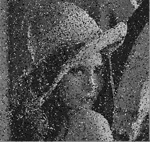
That’s quite different from the output shown from our reference article. So what is wrong?
The answer is: the mode algorithm does not fit to our noise removal issue. Let’s study other algorithms, now that we have grasped a few things and come up with a script we can modify later on!
Median Filter Algorithm
Contrary to the mode filter algorithm, the median filter one consists in taking the median value of our matrix for our filtered pixel.
Back with our matrix:
\[\begin{equation*} \begin{bmatrix} 255 & 102 & 101 \\ 107 & 0 & 105 \\ 106 & 107 & 105 \end{bmatrix} \end{equation*}\]Sorting the values, we have : 0, 101, 102, 105, 105, 106, 107, 107, 255. So we take the value which splits the list in two halfs of same size is 105 :
0, 101, 102, 105, 105, 106, 107, 107, 255.
All we have to do is edit our script to write a simple compute_median function like this:
def compute_median(matrix):
    """Get the median of the *matrix*.

    Just sort the list and get the value at the middle.

    """
    return sorted(matrix)[len(matrix) // 2]
Do not forget to call it instead of compute_median in your previous script. I trust you not to past yet another
script which will likely be the same.
Running the script produces a much better result as you can see:

There are still a couple of trailing, black’n’white pixels here and there, but, hey, it’s much, much better than the mode filter, right?!
Can we do better?!
Mean Filter Algorithm
Even simpler than the previous filters: sum the elements of the matrice, divide by the number of elements and use the result as our pixel value.
Back with our matrix:
\[\begin{equation*} \begin{bmatrix} 255 & 102 & 101 \\ 107 & 0 & 105 \\ 106 & 107 & 105 \end{bmatrix} \end{equation*}\]Summing the values, we have : \(0 + 101 + 102 + 105 + 105 + 106 + 107 + 107 + 255 = 988\)
Then we divide by 9 :
\[988 \div 9 \approx 109\]Our pixel will have the value “109”. Here is our python function:
 def compute_mean(matrix):
    """Get the mean of the *matrix*.

    Sums the element then divide by the number of elements.

    """
    return sum(matrix)//len(matrix)
Running the script does not produce a nice result, but our black’n’white pixels seem to be gone!

So, what’s left?
Gaussian Filter Algorithm
The Gaussian Filter Algorithm is entitled as is from the well known Gaussian function which looks like a bell.
It is similar to the mean filter, where the result pixel is the mean of all of our pixels, but there is a weight applied to our initial pixel’s distance.
As you may have seen in our previous example with the mean filter, the resulting picture have quite some noise. It is because the algorithm does not take into account the pixel’s distance from our result pixel. This is even more problematic in our example where we have this issue of black’n’white pixels we want to get rid of.
Specifically, suppose you are dealing with a “normal pixel” and that there is a either black or white pixel in the resulting 3x3 matrix to apply our filter on. This noisy, black or white pixel will have a significant weight on the resulting mean.
To address this issue, we may use a gaussian function. Bear with me here, because it might make some people run away. Here is our 2D gaussian function:
\[G(x, y) = \frac{1}{2\pi\sigma^2}e^{-\frac{x^2+y^2}{2\sigma^2}}\]Where :
- x and y will be our pixel’s coordinates, relatively to our matrix (NOT the picture!);
- \(\sigma\) (referring to as “sigma” like in the Greek alphabet) is the standard deviation. Its value can be from 1 to the infinite.
But this does not help us much here. What will help us in our algorithm is a 3x3 matrix of coefficients, where the sum of all the elements will be equal to 1.
Let G our matrix to use for the Gaussian filter algorithm. Conventionally, its value will be:
\[G = \frac{1}{16}\begin{equation*} \begin{bmatrix} 1 & 2 & 1 \\ 2 & 4 & 2 \\ 1 & 2 & 1 \end{bmatrix} \end{equation*}\]We can also observe that:
\[\sum_{i=1}^3\sum_{j=1}^3 G_{ij} = 1\]Or, simply put:
\[\frac{1}{16} + \frac{2}{16} + \frac{1}{16} + \frac{2}{16} + \frac{4}{16} + \frac{2}{16} + \frac{1}{16} + \frac{2}{16} + \frac{1}{16} = 1\]How do we put it all together? Well, let’s take back our initial pixel of matrix. Let’s call it P.
\[P = \begin{equation*} \begin{bmatrix} 255 & 102 & 101 \\ 107 & 0 & 105 \\ 106 & 107 & 105 \end{bmatrix} \end{equation*}\]Applying the gaussian filter algorithm, the resulting pixel will be :
\[\sum_{i=1}^3\sum_{j=1}^3 P_{ij} \times G_{ij}\]In our example, letting p being our pixel’s value :
\[\begin{align} p &= \frac{255 \times 1 + 102 \times 2 + 101 \times 1 + 107 \times 2 + 0 \times 4+ 105 \times 2 + 106 \times 1 + 107 \times 2 + 105 \times 1}{16} \\ \\ &= \frac{255 + 204 + 101 + 214 + 0 + 210 + 106 + 214 + 105}{16} \\ \\ &= \frac{1409}{16} \\ \\ &= 88.0625 \\ \\ &\approx 88 \end{align}\]Let’s code our function to get this value.
def compute_gaussian(matrix):
    """Compute the value of our pixel using the gaussian *matrix*.

    Here, we will assume that *matrix* is a list of 9 elements (3x3).

    If the matrix is less than 9 elements, it means that we are at the
    edges of the picture, so we won’t take into account the elements.

    """
    coefficients = {i: matrix[i] if i < len(matrix) else 0 for i in range(9)}
    return int(
        coefficients.get(0, 0) * (1 / 16)
        + coefficients[1] * (2 / 16)
        + coefficients[2] * (1 / 16)
        + coefficients[3] * (2 / 16)
        + coefficients[4] * (4 / 16)
        + coefficients[5] * (2 / 16)
        + coefficients[6] * (1 / 16)
        + coefficients[7] * (2 / 16)
        + coefficients[8] * (1 / 16)
    )
Adjusting the script and running it again produces the result below:
The image still seems noisy, in addition to being blury. Not what I personally expected.
So far, the algorithm that produced the best output is the median algorithm, probably because it reused a value of the picture for our output pixel, so the algorithm to use must depend of the type of noise and the context.
Still, I felt the urge of writing this somewhat incomplete post, as the one I read seemed incomplete to me.
Last but not least, I made the decision to use the pillow library and write some low level algorithms by myself to better understand how the algorithms work, but you may expect the same results by using the numpy and opencv-python libraries!